
10 KPIs indispensables para medir nuestro rendimiento operativo
- Nivel de Calidad Sigma (Sigma Level)
- Tasa de Uso de la Capacidad (CUR, Capacity Utilisation Rate)
- Tiempo de Ciclo de Cumplimiento de los Pedidos (OFCT, Order Fulfilment Cycle Time)
- Tasa de Entrega Completa y A Tiempo (DIFOT, Delivery In Full – On Time)
- Tasa de Contracción del Inventario (ISR,Inventory Shrinkage Rate)
- Rendimiento en la Primera Pasada (FPY, First Pass Yield)
- Nivel de Retrabajo (Rework Level)
- Índice de Calidad (Quality Index)
- Eficiencia General de los Equipos (OEE, Overall Equipment Effectiveness)
- Tiempo de Inactividad de Máquina o Proceso (Process or Machine Downtime Level)

- El producto se encuentre dentro de especificaciones técnicas.
- El producto se entregue en el plazo previsto.
- 400 unidades completas en 18 días
- 160 unidades completas en 24 días
- En el paso A se están produciendo 8 unidades sin problemas, sobre 10 procesadas.
- En el paso B se están produciendo 10 unidades sin problemas, sobre 11 procesadas.
- En el paso C se están produciendo 9 unidades sin problemas, sobre 9 procesadas.
- FPY del paso A (%) = 8 unidades / 10 unidades = 0,8 = 80%
- FPY del paso B (%) = 10 unidades / 11 unidades = 0,9091 = 90,91%
- FPY del paso C (%) = 9 unidades / 9 unidades = 1 = 100%
- PPT que es el tiempo que nosotros planificamos que debe estar operativa una máquina (o un proceso) en un período determinado.
- TA que es el tiempo que realmente estuvo disponible en ese período.
- Tiempo de Actividad (%) = TA / PTT
- Tiempo de Inactividad (%) = 1 – PTT/TA
Continuing with the theme of previous publications, we will analyze in this opportunity 10 KPIs related to the operational operation of the processes, to their performance. They are included in the list of 75 KPIs suggested by the author Bernard Marr in his «Key Performance Indicators: The 75+ Measures Every Manager Needs to Know» from which we have already extracted other indicators. We have selected 10 indicators that we consider fundamental and representative to measure the operational performance of the processes. As we have done, we will try to clarify its purpose and its application through simple examples. The KPIs selected this time are as follows:
– Sigma Quality Level (Sigma Level)
– Capacity Utilization Rate (CUR)
– Order Fulfillment Cycle Time (OFCT)
– Full and On Time Delivery Rate (DIFOT, Delivery In Full – On Time)
– Inventory Shrinkage Rate (ISR)
– First Pass Yield (FPY)
– Rework Level
– Quality Index
– Overall Equipment Effectiveness (OEE)
– Machine Down or Down Time (Process or Machine Downtime Level)
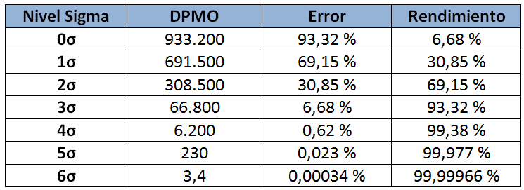
1. Quality Level Sigma (Sigma Quality Level): here the author actually speaks of Six Sigma level, although the correct thing would be to generalize and calculate the level of sigma that our processes have. The sigma level of a process has to do with its efficiency. It is a quantitative measure of the number of defects we produce. In general, the number of defective products per million units produced (DPMO, Defects Per Million Opportunities) is taken into account. Without going deeply into the statistical concept, the level of sigma is related to the number of standard deviations (σ, hence the name) within which our process is. By nature, manufacturing processes tend to have a normal distribution. But, beware, the sigma level of a process is not exactly its standard deviation.
In the following table we can see the acceptable MPD according to the number of «sigmas». The greater number, the better performance we will have. By convention, the following values are adopted.
The number of DPMOs is simple to calculate. It is done as follows:
DPMO = (Number of Defects x 1,000,000) / (Units Produced x Number of Opportunities)
So many units are produced (Units Produced). You get so many defects (Number of Defects) of as many types of defects as possible (Number of Opportunities). The Number of Opportunities tells us how many types of defects we can have.
For example, suppose we produce 7,200 units, of which 435 were defective or non-compliant. Non-conformity, according to our criteria for this case, takes into account that:
The product is within technical specifications.
The product is delivered on time.
That is, the «Number of Opportunities» (the number of possible criteria of nonconformity) is 2. Of the 435 units considered to be defective, 210 are considered noncompliant because they do not meet specifications and the other 225 are out of term. Therefore, the DPMO value of the process will be given by:
DPMO = [(210 + 225) x 1,000,000] / (7,200 x 2) = 30,208.33
If we see in the previous table, we can affirm that our process is between 3σ and 4σ.
As we can appreciate, it is not necessary to produce a million units to obtain our sigma level. It is enough to produce a considerable amount, and extrapolate. There are ways to calculate the exact value of sigma level (with decimals), which gives us a more complete notion of improvement since jumping from one sigma value to another requires a lot of effort. But this will be the subject of a specific publication.
Today in vogue is the application of Six Sigma (Six Sigma). That is, processes that achieve DPMOs less than 3.4. Something achievable for some and utopian for others, but always an excellent north to where to point our efforts. Capacity will be given by: CUR (%) = [(134,542 bottles / hour)] / [(180,000 bottles / hour)] = 74,75% We are taking advantage of practically ¾ of the maximum capacity. Here we must analyze why capacity is reduced and what opportunities for improvement we have.
CUR (%) = (Current capacity in a given period of time) / (Maximum capacity in that period)
If, for example, we make bottles of beer. Our machine is in good condition and is designed to deliver 180,000 bottles in one month (6,000 per day). In the current month 134,542 bottles were produced. The Capacity Utilization Rate will be given by:
CUR (%) = [(134,542 bottles / hour)] / [(180,000 bottles / hour)] = 74.75%
We are taking advantage of ¾ of maximum capacity. Here we must analyze why capacity is reduced and what opportunities for improvement we have.
3. Order Fulfillment Cycle Time (OFCT): As we know, customer satisfaction depends not only on compliance with technical specifications but also on other factors (delivery times, costs, etc.). In this case, the OFCT is an indicator of importance that specifically measures how much time elapses between the customer issuing the order and receiving the product or service that requested. The OFCT will be given by:
OFCT = Materials Reception Time + Production Time + Delivery Time (logistics)
Suppose we receive a customer order for a batch of products. Once confirmed, we proceed to request raw material from a supplier, which takes 5 days. When we receive the raw material we prepare the lot, which takes us 8 days. The customer is 1,000 kilometers, which means an additional 1 day in transportation. That is, since the customer issued the order passed:
OFCT = 5 days + 8 days + 1 day = 14 days
4. Full and On Time Delivery Rate (DIFOT): In relation to the previous indicator, DIFOT gives us an idea of the degree of fulfillment of the orders in time and in form (complete), according to What awaits and what we agree with our client. It is a percentage metric that shows us how much of everything delivered was done on time:
DIFOT (%) = (Number of Units Delivered Complete and in Time) / (Total Units Delivered)
If, for example, our customer asks for 560 units with a maximum term of 20 days but we deliver:
400 complete units in 18 days
160 complete units in 24 days
Our DIFOT will be given by:
DIFOT (%) = 400 units / 560 units = 71.43%
If the delivered units are made on time but are not complete they will also affect the percentage.
5. Inventory Shrinkage Rate (ISR): This is a measure of how our inventory behaves over time. It allows us to know how much is being contracted, reducing, whether due to damage, obsolescence or expiration of the materials contained in it. We know that to operate normally we must have a certain inventory. The Inventory Contraction Rate will be given by:
ISR (%) = (Inventory we should have – Inventory we actually have) / (Inventory we should have)
Suppose that to supply a regular demand, we must have 850 units of certain material in inventory. But part of the inventory is damaged by poor storage, so we have to drop 25 units. We have specifically 825 units available. The Inventory Contraction Rate in this case is:
ISR (%) = (850 units – 825 units) / (850 units) = 2.94%
The higher the ISR value, the greater our inability to keep the inventory under conditions.
6. First Pass Yield (FPY): This is an excellent measure of operational efficiency. It tells us what percentage of products are circulating through the process without problems, subdividing their analysis into steps. It is calculated as:
FPY of step (%) = FPY of step A (%) x FPY of step B (%) x … x FPY of step n (%)
If we have a process that is composed of 3 consecutive steps, of which:
In step A, 8 units are being produced without problems, over 10 processed.
In step B 10 units are being produced without problems, over 11 processed.
In step C 9 units are being produced without problems, over 9 processed.
We will have:
FPY of step A (%) = 8 units / 10 units = 0.8 = 80%
FPY of step B (%) = 10 units / 11 units = 0.9091 = 90.91%
FPY of step C (%) = 9 units / 9 units = 1 = 100%
The FPY of the process will be given by:
FPY of the Process (%) = 0.8 x 0.9091 x 1 = 0.7273 = 72.73%
If we manufacture 1,400 units this month, of which 120 require reprocessing, the Rework Level will be given by:
Rework Level (%) = 120 units / 1,400 units = 8.57%
Of course, the smaller the number, the better and more efficient our process.
8. Quality Index: This indicator does not have a predefined form. It depends heavily on how our process is. The idea is to establish an indicator that represents quantitatively the level of fulfillment of customer expectations, depending on how our product / service fits the purpose, the intended use. This indicator can be calculated as a combination of other indicators, taken with equal weight or weighted according to their importance on the final index.
9. Overall Equipment Effectiveness (OEE): this indicator is one of the most important and used to measure the efficiency of machines and / or processes. It was treated in detail in an earlier publication that we suggest visiting, and that includes an Excel template to calculate it. It is related to three fundamental parameters of a process: availability, performance and quality. You can access this publication in the following link:
What is OEE and how is it calculated? + Excel sample (to download)
10. Process or Machine Downtime Level: is a measure of how much time a machine or process is actually available in an operative manner, with reference to an estimated time of operation. It is usually calculated in two ways. The first, as a percentage (a ratio) between two parameters:
PPT which is the time that we planned that a machine (or a process) must be operative in a certain period.
TA is the time that was actually available in that period.
In this case, one way of measuring Activity (or Inactivity) is:
Activity Time (%) = TA / PTT
Inactivity Time (%) = 1 – PTT / TA
Suppose that in a given month we expected to have a specific machine operative for 200 hours but it worked for 165 hours, as it was stopped mechanically. We will have:
Activity Time (%) = TA / PTT = 165 hours / 200 hours = 82.5%
Or, which stands for the same:
Inactivity Time (%) = 1 TA / PTT = 1 – (165 hours / 200 hours) = 17.5%
It is clear that the activity time should be as high as possible, to comply with what is planned.
The other way of calculating the Inactivity Time is as a simple subtraction between the expected time of activity and the active real time.
Time of inactivity (diff) = PTT – TA
In the previous example:
Time of inactivity (diff) = PTT – TA = 200 hours – 165 hours = 35 hours
NOTE: These KPIs, like the rest of the ones proposed by the author do not necessarily apply to your organization, or are key to your activity. But they can be a very good starting point or a reference to create new indicators.
For more information, we suggest consulting (prior registration) the KPIs online library of the Advanced Performance Institute, directed by Marr himself: http://www.ap-institute.com/kpi-library.aspx
[:]